Calculus: Two Important Theorems – The Squeeze Theorem and Intermediate Value Theorem

By Hannah Gao on 8 Mar 2022 • ( 20 Comments )

Learn about two very cool theorems in calculus using limits and graphing!

The Squeeze Theorem

The squeeze theorem is a useful tool for analyzing the limit of a function at a certain point, often when other methods (such as factoring or multiplying by the conjugate) do not work. This theorem also has other names like the Sandwich Theorem or the Pinch Theorem, but it is most commonly called the Squeeze Theorem.

As mentioned, the squeeze theorem can track the behavior of a function f(x), though there is one caveat: f(x) must be squeezed between 2 other functions.

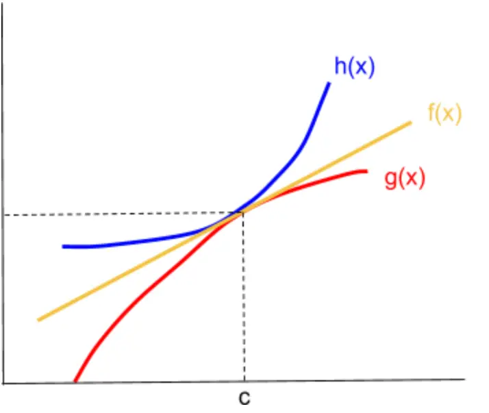
Take a look at the picture below. f(x) is squeezed between h(x) and g(x), and both h and g seem to approach a common y-value at x=c; so it makes sense that f(x) would approach that same y-value at x=c as well.

IMPORTANT!

To put this all into cohesive statement, let’s look at a formal definition for the squeeze theorem:

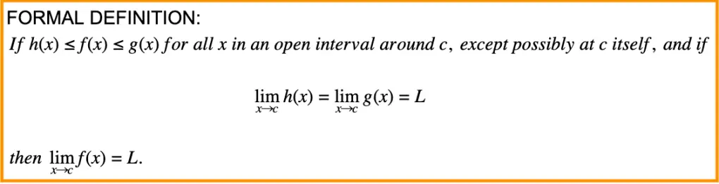
It is important that your function f(x) is always between the other 2 functions h(x) and g(x) on the interval around c, because otherwise we cannot use the “squeezing” argument on f.

It is also crucial to note that the limits of g(x) and h(x) as x approaches c must be equal to each other – if they are not equal, we cannot determine what will happen to the function between them.

From the Squeeze Theorem, we can derive 2 important trigonometric limits:

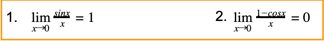
Let’s prove the first one together using the Squeeze Theorem.

Since we need to place upper and lower bounds on our function in order to use the Squeeze Theorem, let’s try to do that.

From the range of sin(x), we know that

If we divide all parts of the inequality by x to produce the function we want to bound, we get

Now, we can take the limit of both sides. Since the limit as x approaches 0 of -1/x and 1/x is 0, we have:

Thus, by the Squeeze Theorem we have proven our first trigonometric identity. Note that this is not the only proof for the Squeeze Theorem – there is actually a more graphical version.

The proof for the second identity is very similar. See if you can do it on your own!

PRACTICE!

Prove the second trigonometric limit. (Hint: use a similar tactic that we used in the first proof; that is, think about the range of cos(x) and try to create bounds)

———————————————————————————————————–

The Intermediate Value Theorem

The Intermediate Value Theorem, often abbreviated as IVT, deals with a single function unlike the Squeeze Theorem.

IMPORTANT!

Here is the formal definition of the Intermediate Value Theorem:

If f(x) is a continuous function on the interval [a, b], and k is a value such that f(a) < k < f(b), then there exists at least 1 value c for which f(c) = k.

To see why this makes logical sense, let’s look at the graph of a function.

The function f(x) shown is continuous on [a, b] and clearly x = c is between a and b. Since f(x) is one smooth curve on the interval, it exhibits no gaps, and therefore it is quite intuitive that f(x) must hit every y-value between f(a) and f(b) at some point between a and b.

It is important to realize that this theorem does not tells us that we have exactly one c-value, but rather it guarantees the existence of at least one.

Let’s see how we can have more than one c-value.

In the diagram above, f(x) is still a continuous function. However, this time, on the interval [a, b], f(x) takes on the value y = k a total of 3 times! At the x-values c1, c2, and c3, f(x) = k, thus the Intermediate Value Theorem does not allow us to conclude that there is only a single c-value. To determine a single c-value, we would need to know some additional information, such as if the function is monotonically increasing or decreasing.

One particular use of the IVT is finding where certain roots of a polynomial equation must exist. Here is an example. Try it on your own first before reading the solution!

EXAMPLE!

Below is a table of values for the continuous function f(x). Determine the minimum number of roots of f.

x	f(x)
0	1
2	3
4	1
6	-5
8	8

Table values for f(x)

Solution:

First, recall that a root will occur when f(x) = 0.

f(x) is a continuous function, so we know that we can use the IVT. We are not given any values of f(x) before x = 0, so we cannot determine anything about its behavior before that. Between x = 0, and x = 2, the IVT does not guarantee a root because f(0) = 1 and f(2) = 3, and 0 is not between 1 and 3 (although the IVT also does not guarantee that there is no root either). Similarly, there is no guarantee of a root between x = 2 and x = 4. However, the IVT guarantees a root between x = 4 and x = 6, because f(4) > 0 > f(6). Similarly, there must be a root of f(x) between x = 6 and x = 8.

Thus, by the Intermediate Value Theorem, there are at least 2 roots for the function f(x).

Remember, there could be more than 2 roots, but given the information we have, we cannot determine any more.

Click and check out these popular articles for more information: 🙂

Should I Take AP Calculus?

AP Calculus Limits and Continuity

Ectoderm vs Endoderm vs Mesoderm

Psychology 101 and the Brain: Stress – Definition, Symptoms, and Health Effects of the Fight-or-Flight Response

Circulatory System: Blood Flow Pathway Through the Heart

Circulatory System: Heart Structures and Functions

Ductus Arteriosus Vs Ductus Venosus Vs Foramen Ovale: Fetal Heart Circulation

Cardiac Arrhythmias: Definition, Types, Symptoms, and Prevention

Upper Vs Lower Respiratory System: Upper vs Lower Respiratory Tract Infections